Usage examples

The procedures and scenarios described in this section illustrate several typical use cases for manipulating neuron morphology reconstructions using the treem module. Ensure that the module is properly installed and accessible. You can verify this by importing it and confirming that no errors are returned:

python3 -c "import treem"

Python version 3.7 or higher is assumed. Ensure that the files from tests/data/ within the module’s source tree are copied into the current working directory.

API use cases

Loading the reconstruction

>>> from treem import Morph
>>> m = Morph('pass_simple_branch.swc')
>>> m.data
array([[ 1. ,  1. ,  0. ,  0. ,  0. ,  1. , -1. ],
       [ 2. ,  3. ,  1. ,  1. ,  0. ,  0.2,  1. ],
       [ 3. ,  3. ,  2. ,  2. ,  0. ,  0.2,  2. ],
       [ 4. ,  3. ,  1. ,  3. ,  0. ,  0.2,  3. ],
       [ 5. ,  3. ,  0. ,  4. ,  0. ,  0.02,  4. ],
       [ 6. ,  3. , -1. ,  5. ,  0. ,  0.2,  5. ],
       [ 7. ,  3. , -2. ,  6. ,  0. ,  0.2,  6. ],
       [ 8. ,  3. ,  3. ,  3. ,  0. ,  0.2,  3. ],
       [ 9. ,  3. ,  4. ,  4. ,  0. ,  0.2,  8. ],
       [10. ,  3. ,  3. ,  5. ,  0. ,  0.2,  9. ],
       [11. ,  3. ,  2. ,  6. ,  0. ,  0.2, 10. ],
       [12. ,  3. ,  5. ,  5. ,  0. ,  0.2,  9. ],
       [13. ,  3. ,  6. ,  6. ,  0. ,  0.2, 12. ]])

Traversing the tree

Traverse the tree starting from the root node.

>>> start_node = m.root
>>> [node.ident() for node in start_node.walk()]
[1, 2, 3, 4, 5, 6, 7, 8, 9, 10, 11, 12, 13]

Traverse the tree starting from the node with ID 8.

>>> start_node = m.node(8)
>>> [node.ident() for node in start_node.walk()]
[8, 9, 10, 11, 12, 13]

By default, the tree is traversed in descending order. In the example above, a subtree (branch) starting at the node with ID 8 is iterated. To traverse the tree in ascending order, set the reverse argument of treem.Node.walk() to True:

>>> [node.ident() for node in start_node.walk(reverse=True)]
[8, 3, 2, 1]

Note that when reverse is enabled, the full tree is not traversed — iteration stops as soon as the root node (ID 1) is reached.

During traversal, data stored at each node can be accessed directly. For example, to calculate the total length of a branch starting from start_node:

>>> sum(node.length() for node in start_node.walk())
8.485281374238571

An alternative way to traverse the tree is by iterating through its sections (in descending order):

>>> for sec in start_node.sections():
>>>     print([node.ident() for node in sec])
[8, 9]
[10, 11]
[12, 13]

The total length of the branch calculated in this way will be identical:

>>> sum(m.length(sec) for sec in start_node.sections())
8.485281374238571

CLI use cases

Checking the input file

Check the input SWC file for structural consistency and compliance with the format requirements defined by the treem module. For example, the records in the file fail_unordered.swc are not in the correct order, so the check command reports errors:

swc check fail_unordered.swc

node1_not_id1: 2
node1_has_parent: 1
node1_not_soma: 3
not_valid_parent_ids: 1

Converting the input file

Attempt to convert the input file to a compliant format. If there are no critical errors in the file structure, the conversion will complete successfully:

swc convert fail_unordered.swc -o out.swc

converted   7%
converted  15%
converted  23%
converted  30%
converted  38%
converted  46%
converted  53%
converted  61%
converted  69%
converted  76%
converted  84%
converted  92%
converted 100%

Verify that the output file is valid:

swc check out.swc

Displaying the morphology

The view command displays the structure of the morphology reconstruction. It renders only the centerline of the reconstructed segments, without showing their diameters:

swc view pass_nmo_1.swc

The root node is displayed as a bold black dot, while soma points are shown as semi-transparent spherical markers. Colored lines correspond to neurites of different types.

To display multiple cells, change the color mode to highlight individual cells:

swc view -c cells pass_mouselight_1.swc pass_mouselight_2.swc

Measuring morphometry of the reconstruction

The measure command prints the basic morphometric features of the reconstruction:

swc measure pass_nmo_1.swc

pass_nmo_1
apic area        12266.1
apic breadth          32
apic contrac    0.932844
apic degree            2
apic diam       0.816706
apic dist        748.044
apic length      5690.72
apic nbranch          31
apic nstem             1
[...]
dend xdim         537.78
dend ydim         332.53
dend zdim          158.9
soma area        3137.66
soma diam         18.246
soma volume      9541.64
soma xroot             0
soma yroot             0
soma zroot             0

Locating single nodes

The find command locates individual nodes that satisfy multiple search criteria. For example, to find a node within the dendrites (point type 3) with a diameter smaller than 0.1 µm, run the following:

swc find pass_simple_branch.swc -p 3 -d 0.1 --comp lt

5

The following command searches for nodes with a topological order of 1 (those belonging to primary neurite sections):

swc find pass_simple_branch.swc -e 1

The following command displays the terminal sections of the dendrites:

swc view pass_simple_branch.swc -b `swc find pass_simple_branch.swc -p 3 -b 1 --sec`

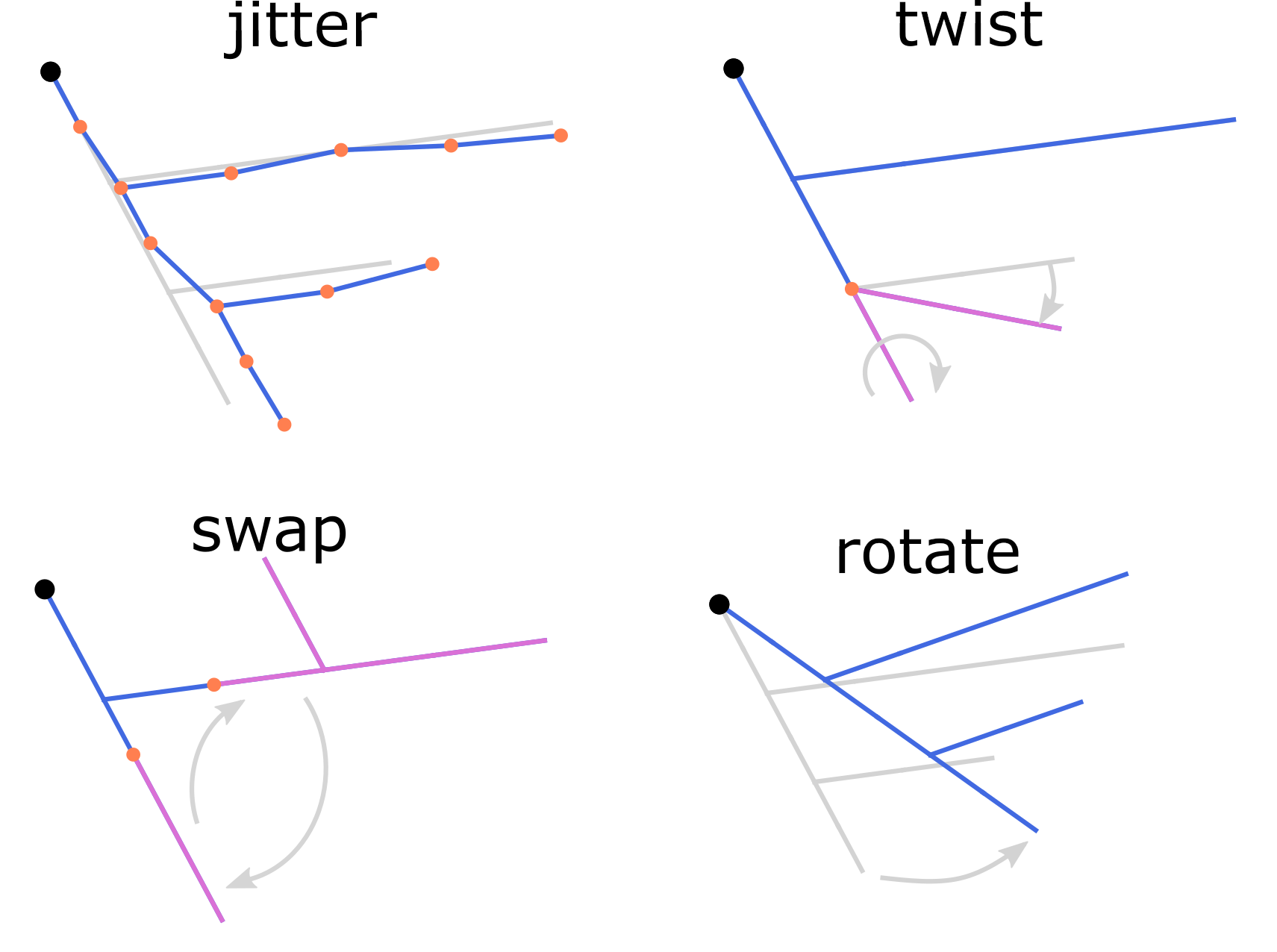
Repairing damaged reconstructions

A common reconstruction error is the so-called z-jump, which occurs when a portion of a neurite is displaced along the z-axis by several micrometers.

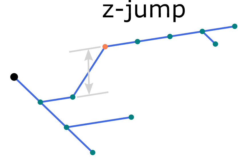
An illustration of z-jump in the morphology reconstruction.

To locate z-jumps greater than 10 µm, run the find command:

swc find pass_zjump.swc -z 10

4

Potential z-jumps can be corrected using the repair command with one of four methods: align, split, tilt, or join (default: align), as illustrated in the figure. To repair z-jumps, run:

swc repair pass_zjump.swc --zjump join -z `swc find pass_zjump.swc -z 10`

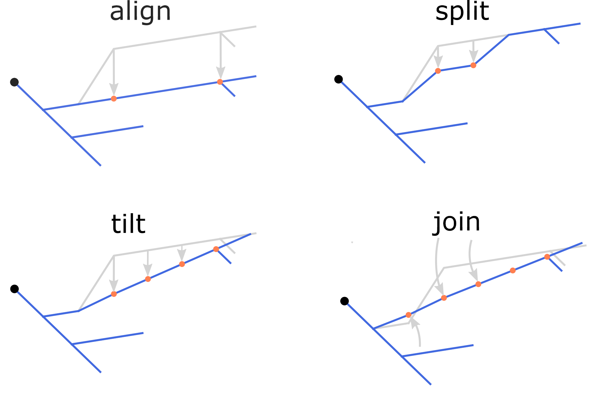
The four methods of correcting z-jumps.

Experimental slice preparation protocols may result in tissue shrinkage. As a consequence, morphology reconstructions appear smaller, with increased neurite contraction compared to in vivo conditions. To compensate for this effect, various options of the repair and modify commands can be used.

Refer to the following options for correction and adjustment:

• -s, -t, and -m (modify command) - scaling, stretching, and smoothing, respectively.

• -k and -kxy (repair command) - shrinkage correction along the z axis and within the (x, y) plane, respectively.

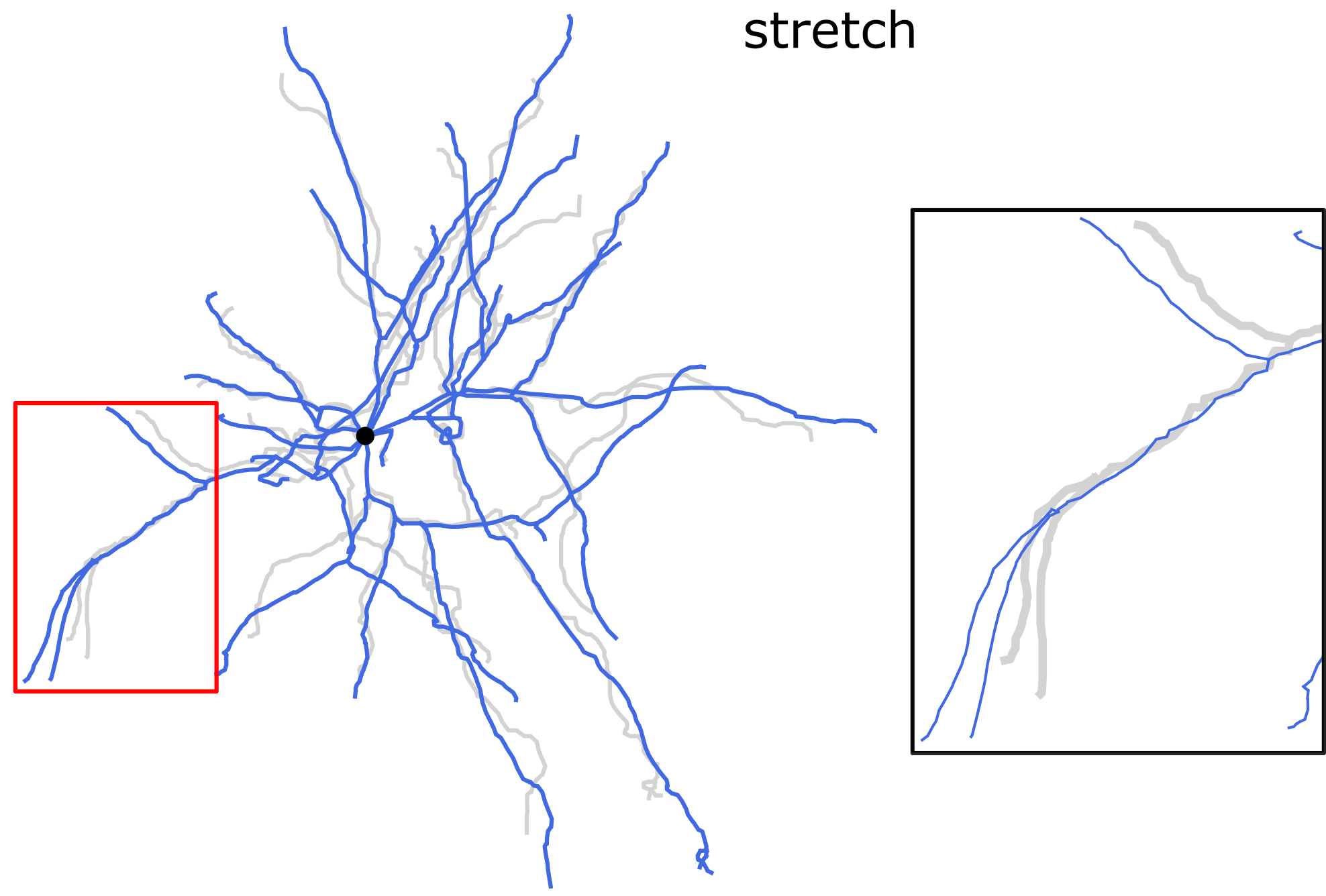
Stretching the dendrites along the direction of each dendritic section. Length-preserving operation.

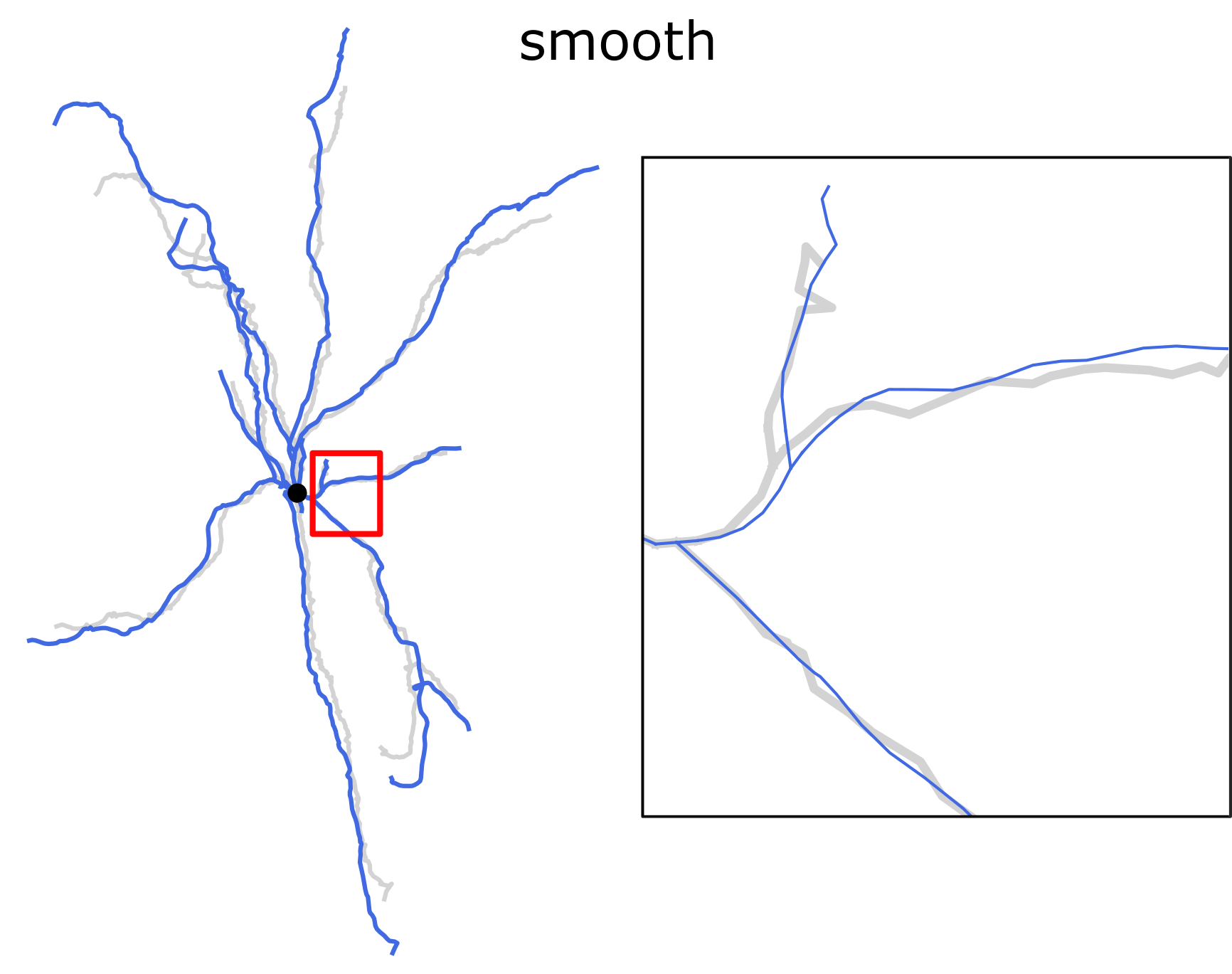
Smoothing the dendrites with the rolling average spatial filter. Length-preserving operation.

Morphological reconstructions of neurons located near the surface of a slice are often incomplete, missing neurites that were cut during tissue sectioning. The cut points of dendrites can be identified using the find command:

swc find pass_nmo_2_cut.swc -c 10 -p 3

322 341 547 1167

In this example, it is assumed that the cut points are located within 10 µm of the top surface of the slice along the z-axis. To invert the surface orientation, add the --bottom-up option.

Inspect the cut points in the projection and note their ID numbers for subsequent repair:

swc view pass_nmo_2_cut.swc -p 3 -j xz --show-id -m `swc find pass_nmo_2_cut.swc -c 10 -p 3`

If all cut points are correctly identified, pass them to the repair procedure:

swc repair pass_nmo_2_cut.swc -c `swc find pass_nmo_2_cut.swc -c 10 -p 3`

Alternatively, specify selected node IDs using the -c option of the repair command.

The repaired reconstruction (rep.swc) can be compared with the original using the view command and the -c shadow option:

swc view pass_nmo_2_cut.swc rep.swc -p 3 -c shadow

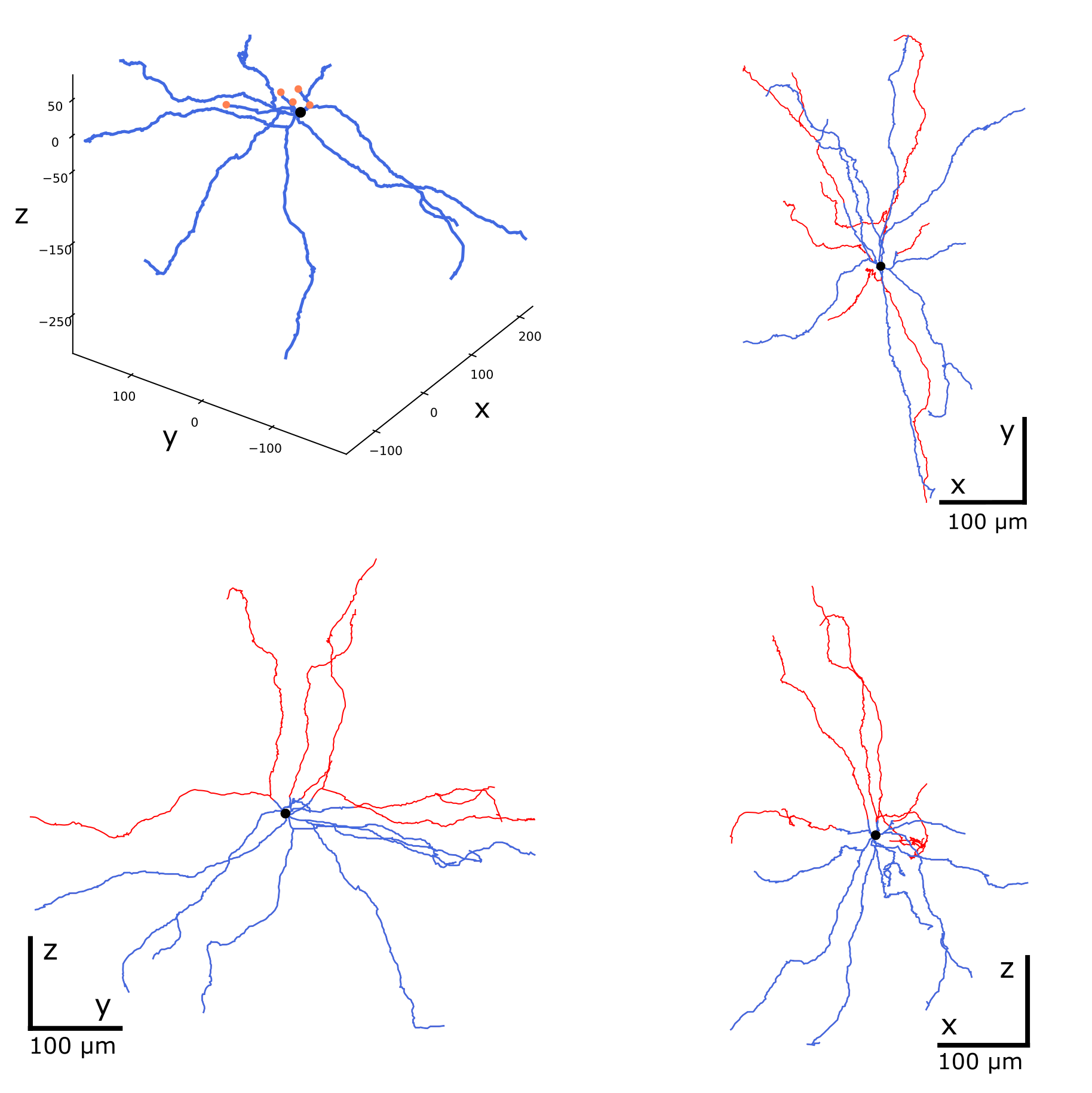
Repairing cut neurites. The cut points are orange, the repaired branches are red.

When the -c shadow option is used, the second and all subsequent morphologies are plotted as underlying structures, with the first morphology rendered on top. The default shadow color is lightgray, and the line width is 3.0. To produce a plot like the one shown in the figure above, run the following command:

swc view pass_nmo_2_cut.swc rep.swc -p 3 -c shadow --shadow-color red --shadow-width 0.5

Modifying morphologies

Corrected or repaired morphology reconstructions may require additional modifications before being used in the simulation pipeline. A common example is cloning the completed reconstructions with random alterations of their neurites. This approach increases variability within the population of morphologies while preserving their topological structure and statistical characteristics, as illustrated in the figure. For details, see the corresponding options of the modify and repair commands.

Length-preserving modifications of the morphology reconstructions.

Morphological modifications are applied to clone existing reconstructions and increase morphological variability in simulations. As an example, consider the random morphology generated by the repair command, as described in the section above:

swc repair pass_nmo_2_cut.swc -c `swc find pass_nmo_2_cut.swc -c 10 -p 3` --seed 123

The default name of the repaired morphology is rep.swc. In this example, the repaired morphology (rep.swc) is modified by twisting its dendrites at the branching points by a random angle of up to ±180 degrees. The resulting morphology (mod.swc) is then scaled in the x, y, and z dimensions by a factor of 0.8. The final structure is saved as clone1.swc:

swc modify rep.swc -p 3 -w 180
swc modify mod.swc -s 0.8 0.8 0.8 -o clone1.swc

Similarly, the dendrites of the reconstruction (rep.swc) are twisted and scaled by a factor of 1.2, producing the morphology clone2.swc:

swc modify rep.swc -p 3 -w 360
swc modify mod.swc -s 1.2 1.2 1.2 -o clone2.swc

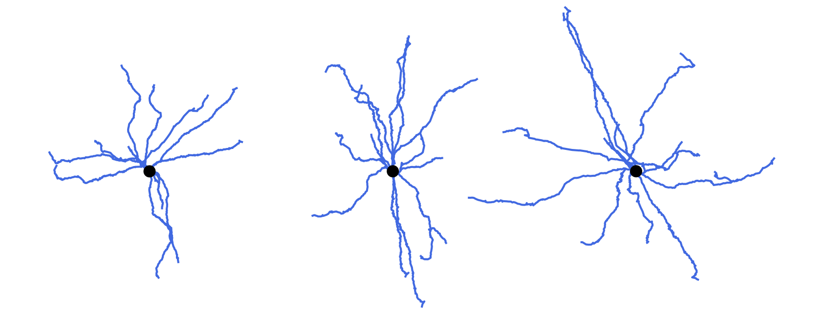
Cloning morphologies with random modifications. Original morphology in the middle. Cloned morphologies have the dendrites twisted randomly at the branching points and scaled by the factor of 0.8 (on the left) and 1.2 (on the right).

Finally, the completed reconstructions can be resampled using a fixed spatial resolution. This operation preserves the positions of the structure-defining points (i.e., neurite stem points, branching points, and terminals) while slightly reducing the total length.

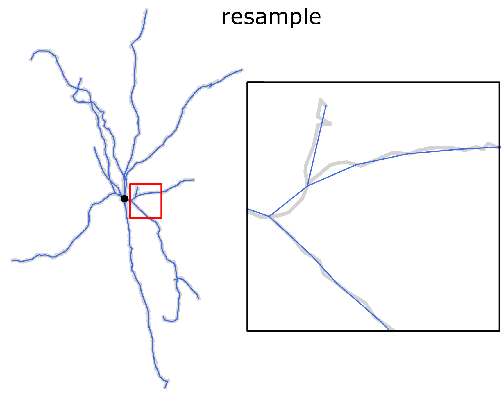
Resampling morphology reconstruction with fixed spatial resolution. Structure points-preserving operation.

For a complete list of the available options provided by the treem module, see Command-line interface and API reference.